Tectonogeomorphic Mapping
We completed surficial mapping of Quaternary alluvium and fault scarps in the Panamint Valley transtensional relay (PVTR, see Figure 2) between December 2020 - March 2022. The map area for this study covers ~40 square kilometers, north of 35°58’0” N, south of 36°3’0” N, east of -117°15’30” W, and west of -117°18’0” W. We completed field and remote mapping of this area at a resolution of 1:4000 using base maps consisting of GeoEye aerial imagery, newly developed 5 cm structure-from-motion (SfM) digital surface models (DSMs), as well as slope and hillshade derivatives from National Center for Airborne Laser Mapping (NCALM) 0.5 m airborne lidar collected from the EarthScope SoCal Lidar Project (Prentice et al., 2009) accessed at OpenTopography (http://opentopography.org). We used this surficial mapping to locate zones with high concentrations of ruptures in late Holocene alluvium, where lidar coverage was often absent, to collect high resolution SfM imagery for remote identification of faults and measurement of offsets.
Developing a Relative Alluvial Fan Stratigraphy
Our surficial mapping involves subdividing generations of alluvial fans based on an extensive set of morphology indicators involving bar and swale morphology, development of desert pavement, weathering of surface clasts and development of soil. We used inset, burial and onlap relationships and relative elevation above the modern wash (Bull, 1991; Spelz et al., 2008) to separate different generations of alluvium. Bar and swale morphologic indicators helped us interpret the relative the age of the surface, which can be used to approximate the age of the underlying deposit. This assumption is violated in the case of a resurfacing event such as a lake highstand or increased plant density (Quade, 2001) as surficial processes can reset, or change the rate of, bar and swale morphology and soil development. Where there is low accommodation space, alluvium can be resurfaced by proximal active washes or thin (< ~.5 m) fan deposition, intermingling and reworking. Where plant density increases closer to active washes or nearer to the playa, there is greater potential for resurfacing through bioturbation.
Bar and Swale Morphology
We used the evolution of braided bar and swale morphologies as a primary indicator for relative alluvium age since these morphologies display fairly consistent changes across different generations of alluvium in Holocene deposits and are the dominant morphology in my field area. Typically, bars consist of coarse gravel to cobble clasts deposited along the edge of flow paths in elongate deposits separated by channels of fine sand, silt, and clays (e.g., Denny, 1965; McFadden et al., 1989; Powell, 1998; Supplemental Figure 1). When deposited in braided systems, coarser clasts group and stack in bars, and develop imbrication in the direction of flow. In between these coarser clasts are open pockets of air and exposed clast edges, referred to as “open-framework” (Tye, 2004; Machette et al., 2008; Regalla et al., 2022). Through time, bar margin-swale contacts become less sharp due to the larger gravitational potential energy stored by coarse-grained sediments in bar crests compared to the finer-grained sediments in proximal swales. As the surface ages, coarser grains roll downhill into the swales, decreasing the average relief of the bar, and reducing the amount of imbrication and stacking of clasts in bars. Additionally, loess infill accumulates at the base and edges of clasts, filling the open-framework by eolian fines, contributing to the decrease in surface relief (Frankel and Dolan, 2007). The morphology indicators that we used to characterize bar and swale morphology include: 1) preservation and sharpness of bar and swale edges, including measurements for uncertainty in this boundary, 2) preservation of depositional imbrication and clast stacking and 3) percentages of secondary loess infill in the open-framework around surface clasts. These processes are complemented by the development of desert pavement described in the following section.
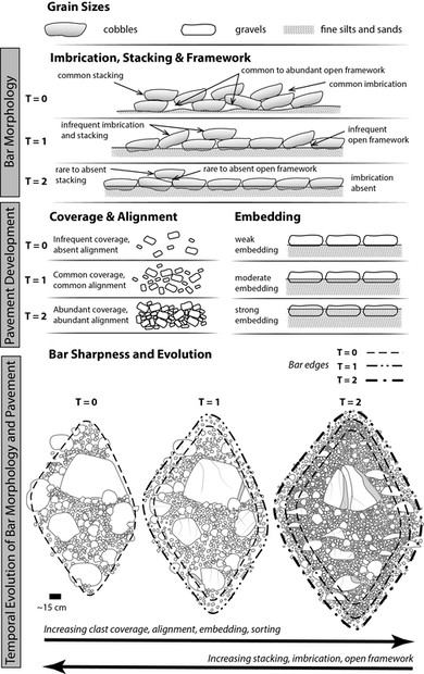
Supplemental Figure 1: Schematic diagram showing examples of different parameters used in this study to assess relative age of desert pavement and bar and swale morphologies. Initial depositional morphologies are shown with T = 0. Additional generic timesteps are shown in T = 1, 2. Abundance terms are defined by the following: absent 0%, rare 0-10%, infrequent 10-40%, common 40-70%, abundant 70-100%.
Desert Pavement Development
Desert pavement was another primary indicator that we weighted heavily in the relative determination of Holocene alluvium age due to fairly consistent changes in pavement development through time. Desert pavements are defined as low-relief, tightly packed, darkly varnished gravels, above a dominantly fine-grained eolian layer (McFadden et al., 1987). Desert pavement forms as eolian influx accumulates below a surficial layer of alluvium, as that surficial layer of alluvium breaks down mechanically and chemically into smaller gravel sized clasts (e.g., McFadden et al., 1987, 2005; Wells et al., 1995; Wood et al., 2005; Matmon et al., 2009). The resulting aggradational surface gradually becomes a loess-cemented, gravel-rich pavement, overlying a secondary layer of eolian fine-grained sands and silts, with strongly developed iron and carbonate rich soils underneath. To define the degree of pavement development, we used four parameters including percentage of clast coverage, interlocking frequency, interlocking strength (i.e., strength of clast embedding), and average clast size (Pietrasiak et al., 2014). We defined four terms for the strength of embedding, ranging from very weak to strong (Figure 4). We define very weak embedding as clasts that mantle the surface but are not physically embedded into the ground, or do not leave an imprint when removed from the surface. We define weak embedding as clasts that leave imprints in the underlying loess but are not cemented into the loess and do not take force to remove. Moderately embedded clasts leave a ≥ 1mm imprint in the ground, but do not disturb other clasts when removed from the loess matrix. Strongly embedded clasts commonly leave a ≥ 3mm imprint in the ground, are difficult to remove from the loess layer (requires some force), and the removal of which disturbs proximal clasts.
Using these terms and parameters, we gave the surface pavement a term to describe the degree of development. Proto-pavements have clasts that begin to mantle the ground and increase clast coverage from ~50-70%, very weakly embedded and infrequently interlocking clasts with a large range in average clast size. Incipient pavements display clasts that have developed a pattern in alignment, some degree of weak embedding and infrequent to common interlocking, a smaller range of ~10 cm in average clast size and a greater degree of clast coverage than proto-pavements. We define moderately developed pavements as having clast mosaics with common clast alignment, moderate-strength embedding with clast sizes reduced to cobbles to coarse gravels and an average range of ~5 cm for average clast size. Strongly developed pavements have strongly developed mosaics with 100% clast coverage, abundant interlocking, and strongly-embedded clasts with average clast sizes <5 cm, with an average size range of 1-3 cm.
Using these terms and parameters, we gave the surface pavement a term to describe the degree of development. Proto-pavements have clasts that begin to mantle the ground and increase clast coverage from ~50-70%, very weakly embedded and infrequently interlocking clasts with a large range in average clast size. Incipient pavements display clasts that have developed a pattern in alignment, some degree of weak embedding and infrequent to common interlocking, a smaller range of ~10 cm in average clast size and a greater degree of clast coverage than proto-pavements. We define moderately developed pavements as having clast mosaics with common clast alignment, moderate-strength embedding with clast sizes reduced to cobbles to coarse gravels and an average range of ~5 cm for average clast size. Strongly developed pavements have strongly developed mosaics with 100% clast coverage, abundant interlocking, and strongly-embedded clasts with average clast sizes <5 cm, with an average size range of 1-3 cm.
Mechanical and Chemical Weathering of Clasts
The mechanical and chemical breakdown of surface rock fragments that comprise bar and swale morphologies display a wider range in disaggregation strength. For this reason, we used parameters describing weathering as a secondary indicator in determining relative age of surfaces. Physical and chemical breakdown of surface clasts is one factor in the development of desert pavement, as clasts experience diurnal temperature variations (Eppes et al., 2010; Eppes and Keanini, 2017), fracture, cleave and disintegrate into gravel to cobble-sized clasts (Figure 4). Clasts in progressively older surfaces show systematic strengthening in several parameters relative to mechanical and/or chemical weathering. These parameters include 1) fracturing, 2) relief involving the disaggregation and grussification of granites, 3) variations in weathering strength of indicators minerals such as micas, feldspars, and quartz, and 4) relief involving the pitting and etching of carbonates. Fracturing is a function of sub-critical cracking at an atomic level (Eppes et al., 2010; Eppes and Keanini, 2017), a process that has been attributed to thermally induced breakdown, or “thermal fatigue” (Molaro et al., 2020) leading to boulder exfoliation and the cleaving of rock surfaces. One unique feature of the older fan surfaces in this study is the presence of ghost boulders (Figure 5), or boulders that have been strongly disaggregated at the surface, rendering the subaerial section of the boulder conical, rounded, or flat while the subsurface section of the boulder is largely preserved (Vidal-Romani and Twidale, 2005).
Soil development
We incorporated a first order description of color, thickness, and carbonate accumulation in soils into surface descriptions, including the A and B horizons where exposed, as a secondary parameter for relative surface age. We used the same color descriptors for B horizons that we used in rubification descriptions. We describe the degree of carbonate accumulation by the amount of clast coverage by carbonate, thickness of the carbonate layer on clasts, and the presence of carbonate filaments or nodules in the fine-grained matrix (Gile et al., 1966; Machette, 1985).
Rupture mapping and Measurement of Offsets
We mapped fault scarps based on the presence of a sharp to degraded topographic surface break, associated with exposure of unvarnished to lightly revarnished rock and soils along slopes. We mapped ruptures using mole tracks, vegetation lineaments, and burrows. Surface ruptures disturb the soil profile, bringing unconsolidated, permeable sediment to the surface, which accumulates moisture and is utilized by vegetation and animals. We located ruptures in older surfaces where they produce a break in the strongly varnished and pavemented surface, exposing freshly unvarnished clast faces and distinct varnish rings on scarp clasts. Varnish rings are a sharp boundary between the varnished surface and the newly exposed, unvarnished underside of a clast on a scarp, indicating the original position of the ground surface prior to rupture (Smith, 1979; Lubetkin and Clark, 1988). Additionally, we traced ruptures from older (Pleistocene) surfaces into the younger late Holocene deposits to find rupture traces in young alluvium.
After mapping ruptures in late Holocene deposits, we measured lateral offsets using piercing points defined by the intersection of bar edges and crests, swale thalwegs and terraces risers with the fault trace to determine the number of events, the slip magnitude per event, and the offset kinematics. We did not measure vertical offset in the field due to the difficulties in matching offset points where bar and swale morphologies change elevation parallel to the scarp. Additionally, field measurements of small vertical offsets (< ~.2 cm) would return uncertainties larger than the amount of offset, making cross correlation of topography from high-resolution DSMs a more favorable method for measuring vertical offset. We measured vertical and lateral offset using LaDiCaoz_v2, a MATLAB-based graphic user interface (GUI), to cross-correlate high resolution topographic data and ‘backslip’ these geomorphic features to calculate a total displacement (Zielke and Arrowsmith, 2012; Haddon et al., 2016). LaDiCaoz_v2.1 generates a unique probability density function (PDF) by cross-correlating topography on opposite sides of a fault using relief, width, and degree of symmetry (Zielke and Arrowsmith, 2012; Haddon et al., 2016). This tool helped me to identify and measure small (< 1 m) total offsets in short wavelength (1 – 2 m) topography that are difficult to recognize in the field.
After mapping ruptures in late Holocene deposits, we measured lateral offsets using piercing points defined by the intersection of bar edges and crests, swale thalwegs and terraces risers with the fault trace to determine the number of events, the slip magnitude per event, and the offset kinematics. We did not measure vertical offset in the field due to the difficulties in matching offset points where bar and swale morphologies change elevation parallel to the scarp. Additionally, field measurements of small vertical offsets (< ~.2 cm) would return uncertainties larger than the amount of offset, making cross correlation of topography from high-resolution DSMs a more favorable method for measuring vertical offset. We measured vertical and lateral offset using LaDiCaoz_v2, a MATLAB-based graphic user interface (GUI), to cross-correlate high resolution topographic data and ‘backslip’ these geomorphic features to calculate a total displacement (Zielke and Arrowsmith, 2012; Haddon et al., 2016). LaDiCaoz_v2.1 generates a unique probability density function (PDF) by cross-correlating topography on opposite sides of a fault using relief, width, and degree of symmetry (Zielke and Arrowsmith, 2012; Haddon et al., 2016). This tool helped me to identify and measure small (< 1 m) total offsets in short wavelength (1 – 2 m) topography that are difficult to recognize in the field.
Backslipped Offsets and Probability Density Functions (PDFs)
We used our newly developed 0.5 cm DSMs to statistically evaluate backslipped reconstructions of offset geomorphic landforms (e.g., Zielke et al., 2012; Haddon et al., 2015) where smaller (~.5 - 1 m) offsets in smaller wavelength (1 – 2 m) bar and swale topography cannot be resolved using the regional NCALM .5 m lidar. We defined the fault trace, and two topographic profiles parallel to the fault trace, from north to south to isolate either the topographic profile associated with a single offset geomorphic landform, or landforms. The down-slope topographic profile (B-B’; Supplemental Figure 2) is then clipped to isolate the landform(s), and cross correlated to topography along the up-slope topographic profile (A-A'). We used a .5 m swath around each profile line to produce a topographic profile with a range of elevation values to account for surface variability. We varied the distance from the fault trace to the profile lines to 1) avoid the topographic signature of vegetation, that causes large spikes in the elevation and greater uncertainty in backslipped reconstructions and 2) to avoid the elevation change due to degradation of the scarp face that could return a smaller (or larger) value than the true total offset. We cropped the up-fault profile to isolate the sharpest, most distinct parts of a geomorphic piercing point. For these reconstructions, we traced the best fit line of the longitudinal profile (vertical projection) into the fault. For each backslip function, we determined a minimum, most likely and maximum total displacement. For each identified piercing point, We repeated the backslip function between 5-8 times to account for uncertainty in reconstruction of the geomorphic feature. We averaged all repeated runs of lateral offset for a single offset feature to get a PDF curve. We report vertical offset as a percentage of horizontal offset for each location. As with the field measurements, We assigned confidence ratings to backslipped features from 1(lowest confidence) to 3(highest confidence), which we used to scale PDFs for cumulative offset probability distribution (COPD) curves.
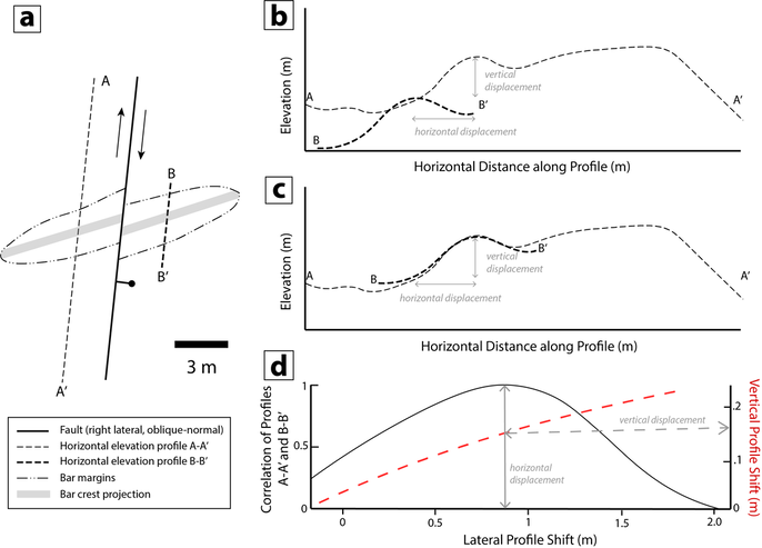
Supplemental Figure 2: A schematic diagram showing the method for reconstructing offset magnitudes from displaced geomorphic markers, using LaDiCaoz_v2 (Zielke et al., 2012; Haddon et al., 2016). We use this script to determine best-fit lateral and vertical displacement by cross-correlating topographic profiles perpendicular to the orientation of the geomorphic feature on either side of the fault A. We define the fault (solid line) and the geomorphic profile of the bar on the western side of the fault (A-A’) and the eastern side of the fault (B-B’). B. Topographic profiles A-A’ and B-B’ before lateral and vertical shift. C. Topographic profiles A-A’ and B-B’ after lateral and vertical shift. D. By mathematically restoring the offset geomorphic marker, the program generates a lateral shift-correlation plot that predicts a most likely displacement for a piercing point. The vertical offset is found by finding the amount of vertical shift necessary to achieve a correlation coefficient of 1 on the lateral profile shift line.
COPD Curves
We used COPD analysis to determine the magnitude of offset along individual surface ruptures and as a first order approximation for the number of earthquakes. COPD curves are plots constructed from summing a set of PDFs that define mathematically calculated offset distributions for a single piercing point. Clusters of offsets create peaks in the COPD plots, used to find the value of likely offsets associated with discrete events. The peaks of PDF and COPD plots represent the probability of an offset value, with the width of the curve representing the uncertainty. Single PDFs report the probability for one offset, and thus will not exceed 1. COPD plots are a sum of all PDFs, with each scaled PDF assigned a confidence level of 1 to 3 (this study), in which the probability of an offset may exceed 1. COPD plots have been used successfully to find the amount of slip per event on faults in southern California (McGill and Sieh, 1991; Madden et al., 2013; Haddon et al., 2016). We generated COPD curves for field offsets and LaDiCaoz_v2 backslipped offsets separately, grouping offset data by age. We filtered data to reduce noise by removing any offsets with a confidence of 1 or 1.5, and s > .25, .20 and .15, that is we removed data that has an uncertainty larger than the offset value. We generated COPD plots for fan ages Qf7, Qf6a, Qf6b, and all fan ages younger than Qf6b, omitting offsets in fans older than Qf6b due to temporal uncertainty in rupture age.
Dating of Offset Deposits
We used luminescence dating to bracket the timing of late Holocene paleoruptures and provide ages for alluvium to further constrain surficial relative dating techniques. For sample dating, we used potassium feldspar post-infrared infrared-stimulated luminescence (pIR-IRSL) recovered from fine sands in ponded sediments and alluvial fans. Luminescence dating works by taking advantage of crystal lattice defects present in silicate minerals such as quartz and feldspar, formed during crystallization (Forman, 2015; Nelson et al., 2015; Feathers, 2020). Background ionizing radiation produces electron vacancies and mobile electrons that may fill some of these defects (Forman, 2015; Nelson et al., 2015; Feathers, 2020). Over time, some of these defects become electron “traps”, unless sufficient heat or sunlight is present to release electrons back to ground state (Forman, 2015; Feathers, 2020). The accumulated energy is proportional to time by the equation: Age = De/Dr, where De is equal to the equivalent dose of mineral grains and Dr is the environmental dose rate (Forman, 2015; Nelson et al., 2015; Zhang and Li, 2020; Feathers, 2020). The equivalent dosage is the amount of radiation required to produce the amount of trapped charge, measured in K-feldspar by the number of photons emitted by the mineral after exposure to infrared light (Nelson et al., 2015; Feathers, 2020). The natural dose rate is the background radiation produced mainly by the decay of U, Th and K present in alluvium (Zhang and Li, 2020). Traditional K-feldspar IRSL displays “anomalous fading”, where electrons from higher energy traps transfer to lower energy traps under ambient temperatures, possibly related to quantum tunnelling (Wintle, 1977; Spooner, 1992, 1994). Post IR-IRSL uses a multi-step IR stimulation process to remove the anomalous fading signal (Zhang and Li, 2020) and find the best electron trap energy that produces reliable luminescence ages.
We used pIR-IRSL because it has been successfully used to date alluvium in the Mohave region (McGuire and Rhodes, 2015; Carr et al., 2019; Regalla et al., 2022), and has provided more reliable ages than optically stimulated luminescence (OSL) on quartz in the Mojave region of southwestern U.S. (Roder et al., 2012; Carr et al., 2019; Zhang and Li, 2020), and organic material needed for 14C dating is not present in the study area.
We used pIR-IRSL because it has been successfully used to date alluvium in the Mohave region (McGuire and Rhodes, 2015; Carr et al., 2019; Regalla et al., 2022), and has provided more reliable ages than optically stimulated luminescence (OSL) on quartz in the Mojave region of southwestern U.S. (Roder et al., 2012; Carr et al., 2019; Zhang and Li, 2020), and organic material needed for 14C dating is not present in the study area.
